Formaldehyde: Geometry Optimization and Vibrations
This example takes formaldehyde from a rough starting structure to its equilibrium geometry, then computes the harmonic vibrational frequencies, the zero-point energy, and the enthalpy and Gibbs free energy at 298.15 K. These two steps are the usual start of any reaction-energy or spectroscopy study.
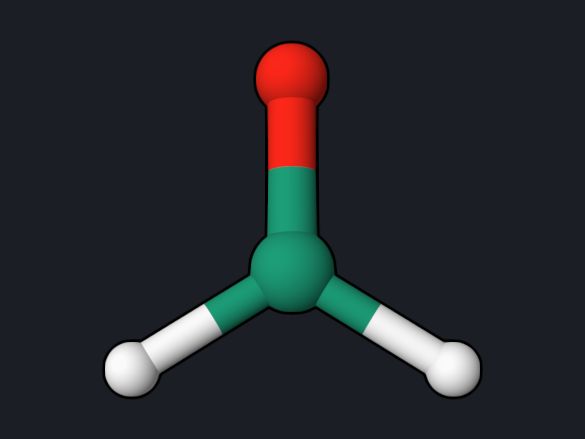
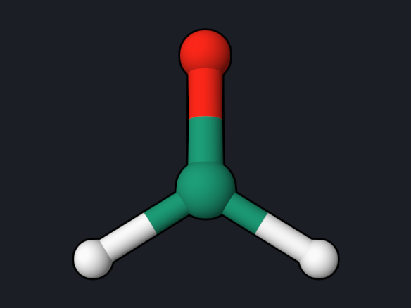
Step 1: optimize the geometry
dft/pbe0/6-31g* opt
geom="""
C      0.000000     0.000000    -0.530000
O      0.000000     0.000000     0.680000
H      0.000000     0.940000    -1.120000
H      0.000000    -0.940000    -1.120000
"""
openqp formaldehyde-opt.oqp
opt asks for a ground-state geometry optimization; the convergence criteria
and step control are defaults. The run takes about 6 seconds and writes the
step table to opt_status.txt:
 Step           Energy            Shift      RMSD Step       Max Step      RMSD Grad       Max Grad
----------------------------------------------------------------------------------------------------------------------
    1    -114.36792361    -114.36792361       0.000000       0.000000       0.005160       0.012676
    2    -114.36801315      -0.00008953       0.003882       0.011249       0.000652       0.001953
    3    -114.36801738      -0.00000423       0.001196       0.002725       0.000187       0.000524
    4    -114.36801804      -0.00000065       0.000672       0.001016       0.000100       0.000291
    5    -114.36801809      -0.00000005       0.000169       0.000341       0.000017       0.000045
The log reports PyOQP: Geometry Optimization Has Converged, and the final
structure is written to opt.xyz. Gradients are in hartree/bohr and steps in
ångström.
| Quantity | Reference value |
|---|---|
| Final energy | −114.3680181 hartree |
| Optimization steps | 5 |
| r(C=O) | 1.2025 Å |
| r(C–H) | 1.1097 Å |
| ∠H–C–H | 115.33° |
Step 2: frequencies and thermochemistry
Use the optimized coordinates from opt.xyz. Frequencies are meaningful only
at a stationary point, so always optimize first with the same method and basis
set.
dft/pbe0/6-31g* hess(S0,type=analytical) ir raman
geom="""
C      0.000000     0.000000    -0.526342
O      0.000000     0.000000     0.676110
H      0.000000     0.937620    -1.119884
H      0.000000    -0.937620    -1.119884
"""
Download formaldehyde-freq.oqp
openqp formaldehyde-freq.oqp
hess(S0,type=analytical) computes the analytic second derivatives of the
ground-state energy. ir raman also requests the dipole and polarizability
derivatives. The run takes about 12 seconds.
| Mode | Symmetry | Frequency (cm⁻¹) | Motion | Experiment (cm⁻¹) |
|---|---|---|---|---|
| 1 | b1 | 1203.45 | out-of-plane wag | 1167 |
| 2 | b2 | 1281.24 | CH₂ rock | 1249 |
| 3 | a1 | 1563.39 | CH₂ scissor | 1500 |
| 4 | a1 | 1882.16 | C=O stretch | 1746 |
| 5 | a1 | 2944.35 | symmetric C–H stretch | 2782 |
| 6 | b2 | 2999.92 | antisymmetric C–H stretch | 2843 |
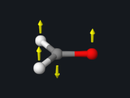
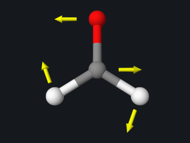
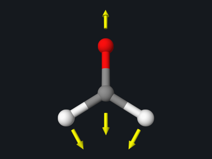
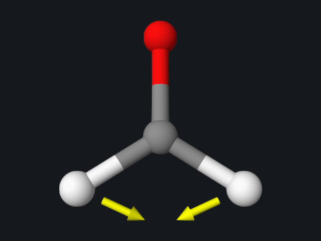
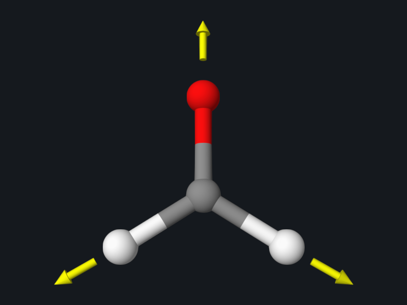
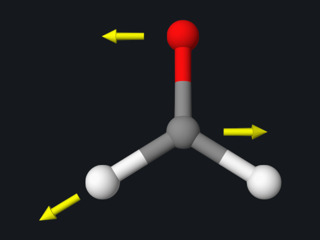
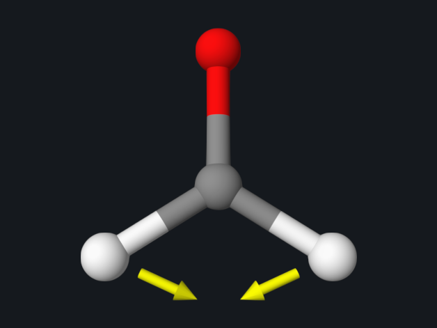
The arrows show the direction in which each atom moves in the normal mode (the out-of-plane wag is viewed from the side).
The experimental values are the observed gas-phase fundamentals. Computed harmonic frequencies are systematically higher, because the calculation omits anharmonicity; a scale factor of about 0.95 is commonly applied before comparison with experiment.
All six frequencies are real (positive), so the optimized structure is a minimum. A negative value in this table would mean an imaginary frequency, that is, a saddle point; see the transition-state example.
The thermochemistry block at the end of the log gives, at 298.15 K and 1 atm:
| Quantity | Reference value |
|---|---|
| Zero-point energy | 0.02705217 hartree (16.98 kcal/mol) |
| Enthalpy H | −114.33715582 hartree |
| Entropy term T·S | 0.02481901 hartree |
| Gibbs free energy G | −114.36197483 hartree |
IR and Raman spectra
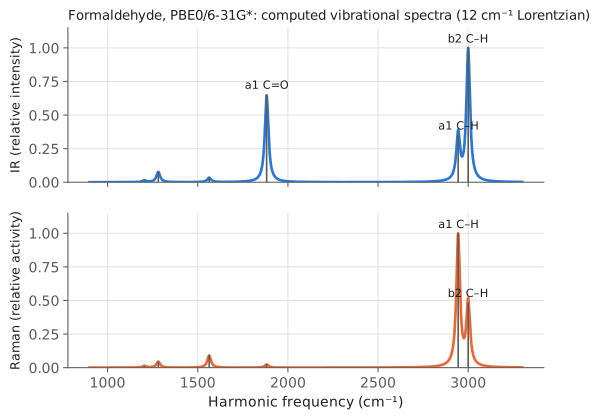
Both spectra are normalized to their strongest band, so they show relative intensities only. The two techniques highlight different modes: in IR the antisymmetric C–H stretch and the C=O stretch are the strongest bands, while in Raman the symmetric C–H stretch dominates.
The absolute values are in the log:
   Mode  Symmetry     Frequency(cm-1)      IR(km/mol)      Raman(bohr^4/amu)
      1        b1           1203.45         2.036547            26.254348
      2        b2           1281.24        12.121916            89.365011
      3        a1           1563.39         5.314512           181.220376
      4        a1           1882.16       102.561925            47.219241
      5        a1           2944.35        55.281427          1953.035868
      6        b2           2999.92       156.454211           949.575196
| Mode | IR intensity (km/mol) | PySCF 2.13 (km/mol) |
|---|---|---|
| 1 · out-of-plane wag | 2.04 | 2.04 |
| 2 · CH₂ rock | 12.1 | 12.1 |
| 3 · CH₂ scissor | 5.31 | 5.40 |
| 4 · C=O stretch | 102.6 | 102.5 |
| 5 · symmetric C–H stretch | 55.3 | 55.3 |
| 6 · antisymmetric C–H stretch | 156.5 | 156.3 |
IR intensities in OpenQP 1.3.1 and earlier
Builds before
openqp#533
(merged 20 October 2026) print an IR(km/mol) column that is 23.07 times
too small, because the conversion factor for (D/Å)²/amu was applied to
atomic-unit dipole derivatives, and label the Raman column Raman(activity).
Relative intensities and all other values are the same. The absolute values
above come from GitHub main commit 0b75a06, which includes the fix.
Look at the vibrations
The run writes formaldehyde-freq.freq.molden and
formaldehyde-freq.hess.json. Open either file in OQP Studio
Analysis or OpenqpView
to animate each normal mode; the C=O stretching mode is shown above.
Cross-check
PySCF 2.13 (PBE0/6-31G* with Cartesian d functions, analytic Hessian) at the same geometry gives frequencies within 2 cm⁻¹ of the values above, and IR intensities from finite-difference dipole derivatives within 2 % (table above). The small differences come from the DFT integration grid.
Try next
- Start the optimization from your own guess, for example a structure with r(C=O) = 1.4 Å, and see how many steps it needs.
See also: Optimization, Hessian and Frequencies, Orbital and Vibrational Output.
Scientific references
Geometry optimization and reaction paths; Vibrational and magnetic properties.